Understanding Embeddings, Similarity Metrics and much more

In the previous blog, we explored the core components of Retrieval-Augmented Generation (RAG). Now, we’ll dive deeper into the embedding process, the significance of magnitude and direction, and how different similarity metrics impact retrieval.

1. The Embedding Process:

When you input a sentence like “The cat sat on the mat” into a transformer model, here’s what happens:

1.  Tokenization:
   Text → `[“The”, “cat”, “sat”, “on”, “the”, “mat”]`
2.  Neural Network Processing:
   Tokens → Mathematical representations
3.  Output:
   A vector such as:
   `[0.23, -0.15, 0.87, 0.02, -0.45, …, 0.33]`

What Do These Numbers Represent?

Each number in the vector corresponds to a dimension that captures semantic features:

• Dimension 1 (0.23): May reflect “animal-ness”
• Dimension 2 (-0.15): Could represent “action vs. state”
• Dimension 3 (0.87): Might encode “domestic setting”
• .. and so on for all 768+ dimensions**

Note: These meanings are not explicitly defined. Neural networks learn them automatically during training.

So, while we can’t know exactly what each number means, we understand that together they represent the semantic fingerprint of the input.

Why Are Embeddings Useful?

Imagine a chatbot helping users with train schedules. A traditional FAQ-based bot only matches pre-written questions. It doesn’t understand the meaning.

With RAG, we improve this:

1.  Parse documents (like train schedules).
2.  Generate embeddings using a transformer
3.  Store these vectors in a vector database (e.g., Pinecone, Weaviate, FAISS)
4.  Embed the user query
5.  Compare embeddings to find the most semantically relevant document

But before comparing vectors, we must understand magnitude and direction.

Understanding Vector Magnitude:

Magnitude is the length of a vector — from its origin to its endpoint.

Formula:

||v|| = √(v₁² + v₂² + v₃² + … + vₙ²)

Example:

• Vector A [3,4] → Magnitude = √(3² + 4²) = √25 = 5
• Vector B [4,1] → Magnitude = √(4² + 1²) = √17 ≈ 4.12

What Does Magnitude Mean in NLP?

Higher magnitude could imply:

• Richer, more complex text
• Stronger semantic features
• More confident predictions

Lower magnitude might mean:

• Short or generic content
• Less semantic richness
• Ambiguity or uncertainty

Example:

Text: “Hello”
Embedding: [0.1, 0.05, -0.02, 0.08, …]
Magnitude: 1.2 (low)

Text: “The physicist explained quantum entanglement…”
Embedding: [0.45, -0.32, 0.67, -0.23, …]
Magnitude: 3.8 (high)

Understanding magnitude can help with:

1. Debugging embedding quality
2. Choosing similarity metrics
3. Optimizing retrieval thresholds

Direction: The True Semantics of a Vector

Vector direction indicates the semantic meaning — the topic or context — that a vector points toward.

Imagine each vector as an arrow from the origin in a high-dimensional space. Two vectors pointing in the same direction mean the texts are semantically similar, even if one is longer (more confident or detailed).

Think of direction as “what you’re talking about“, and magnitude as “how strongly you’re talking about it.“[1]

2. Choosing the Right Similarity Metric:

RAG systems retrieve documents based on vector similarity. Let’s explore three popular metrics:

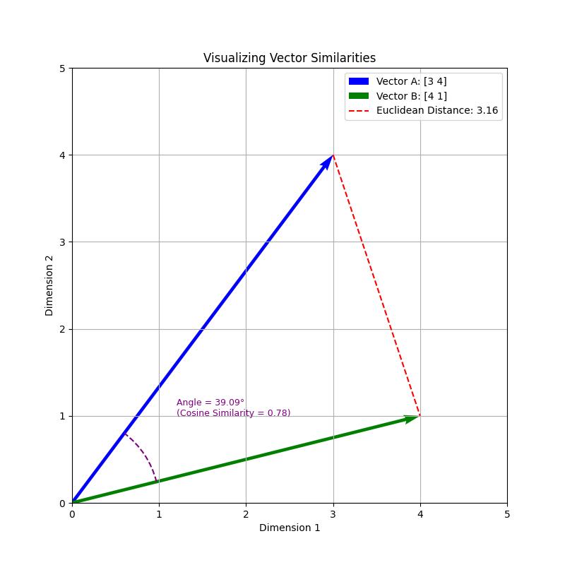Figure 1: Visual representation of Vector A [3,4] and Vector B [4,1] in 2D space. The blue arrow represents Vector A, while the green arrow represents Vector B. The red dotted line shows the Euclidean distance between the endpoints (3.16). The purple arc illustrates the angle between the vectors (39.09°), which corresponds to a cosine similarity of 0.78.

1. Euclidean Distance

What it measures: Straight-line distance between two vectors

• Sensitive to magnitude
• Captures both direction + length
• It can be misleading if documents have the same meaning but different verbosity
• Magnitude Sensitivity: High
• Direction Sensitivity: Moderate

Best Use Case: Image similarity, basic document matching and recommendation system

Formula:

Euclidean Distance = √(a1 – b1)^2 + (a2 – b2)^2 + …. + (an – bn)^2

Distance between A [3,4] and B [4,1]} = √(3-4)^2 + (4-1)^2 = √10 ≈ 3.16

2. Cosine Similarity

What it measures: Angle between two vectors, ignores magnitude

• Focuses on semantic direction
• Most reliable for textual embeddings
• Widely used in modern RAG setups
• Magnitude Sensitivity: None
• Direction Sensitivity: High

Best Use Case: Semantic search, NLP

Formula:
cos(θ)= A⋅B / ∣∣A∣∣ x ∣∣B∣∣

• Cos(0°) = 1 → identical direction
• Cos(90°) = 0 → no similarity
• Cos(180°) = -1 → opposite meanings

Example: Cosine similarity between A and B ≈ 0.78 — they’re quite similar!

3. Dot Product

What it measures: Magnitude + directional alignment

• Rewards high confidence (long vectors)
• Useful when magnitude carries meaning
• Not normalized — can inflate scores
• Magnitude Sensitivity: High
• Direction Sensitivity: High

Best Use Case: When magnitude matters (e.g., ranking)

Formula:

A . B = (3×4) + (4×1) = 12 + 4 = 16

Why Cosine Similarity Wins for RAG

Imagine Vector A was [6,8] (same direction, longer length). Here’s what changes:

• Euclidean distance: Increases
• Dot product: Quadruples
• Cosine similarity: Stays the same

That consistency makes cosine similarity ideal for semantic retrieval, where direction matters more than magnitude. Also, the value of cosine similarity ranges from- 1 to 1. In contrast, Euclidean distance ranges from 0 to infinity, and the dot product can range from negative to positive infinity depending on both the direction and magnitude of the vectors. Cosine similarity avoids this issue, offering a stable and interpretable similarity score that works well for thresholding or reranking in retrieval-based systems[2].

High-Dimensional Reality

Visuals like [3,4] and [4,1] help us grasp the idea. But real models operate in:

• BERT: 768 dimensions
• OpenAI Ada-002: 1536 dimensions
• Newer models: Up to 2560+

Yet the same principles apply:

• Direction = meaning
• Magnitude = strength
• Cosine similarity = best semantic match

Returning to our train scheduler example, using cosine similarity for retrieval would ensure that queries like ‘When does the train to Boston leave?’ and ‘What time is the Boston departure?’ retrieve the same relevant information despite different phrasing. Meanwhile, appropriate chunking strategies ensure that related information (like departure time, platform number, and any service changes) remains connected in the retrieved content.

3. Chunking Strategies for Better Retrieval

While embeddings and selecting the right similarity metrics are critical for semantic retrieval, the quality and structure of the chunks we’re comparing are equally important.

Chunking is the process of splitting large documents into smaller pieces before embedding. Effective chunking maximizes both retrieval accuracy and semantic coverage.

Let’s explore how chunking has evolved, and how these strategies can improve RAG systems.

Syntactic vs. Semantic Chunking

There are two primary approaches:

1. Syntactic Chunking

• Breaks text using natural language structures: paragraphs, sentences, punctuation.
• Easy to implement, linguistically coherent.
• May miss relationships that span across paragraphs.

Example: A paragraph boundary might split related concepts, causing incomplete retrieval.

2. Semantic Chunking

• Groups text based on meaning, not structure.
• Uses techniques like embedding similarity, topic modelling, or clustering.
• Captures thematic cohesion, making it ideal for tasks like question answering, summarization, or context-aware search.

Example: In a legal document, all clauses related to “liability” may be spread across different sections. Semantic chunking can group them together for accurate retrieval[3].

Overlapping Windows & Sliding Techniques

Chunking inevitably cuts documents at certain points. But what happens when a sentence or idea starts near the end of one chunk and continues into the next? This can lead to incomplete retrieval or fragmented understanding. Even with good semantic grouping, the end of one idea might gradually transition into the next, and the chunking algorithm may assign that boundary to one side or the other.

Overlapping strategies help bridge this grey area, ensuring that no key idea gets accidentally cut off. Techniques such as sliding windows and variable overlap are commonly used to address this challenge.

1. Sliding Window

A fixed-size window (e.g., 200 tokens) slides through the text with a stride (e.g., 100 tokens).
This creates overlapping chunks where each piece shares content with its neighbors[4].

This redundancy helps retain information that would otherwise be lost at chunk edges.

2. Variable Overlap

Instead of a fixed stride, the system adjusts overlap dynamically, based on:

• Heuristics or Manual Rules:
  Use cues like named entities near chunk boundaries, high TF-IDF keywords, or punctuation that indicates incomplete thoughts (e.g., commas or conjunctions).
• Embedding-Based Semantic Shifts:
  Take a base chunk size (e.g., 300 tokens), then extract the last 100 tokens of the current chunk and the first 100 tokens of the next chunk. Compute embeddings of these windows and measure cosine similarity.
  • High similarity → smaller overlap needed
  • Low similarity → larger overlap to retain context
• ML / LLM-Based Models:                                                                                                                                                      Use trained classifiers or language models to decide if a boundary is semantically important enough to warrant increased overlap.

This ensures important or high-value content appears in multiple chunks, enhancing recall[5].

Benefits:

• Reduces fragmentation of ideas
• Increases robustness in retrieval
• Improves recall for context-sensitive queries

Choosing the right chunk size is a balancing act:

Small Chunks:

• Higher precision.
• May lose context.

Large Chunks:

• More context.
• May dilute relevance and increase noise.

Need for Adaptive Chunking

Most chunking strategies apply uniformly to all queries, but user queries vary widely:

1. Some queries are broad and exploratory, requiring rich context
2. Others are narrow and specific, needing precise information

Adaptive Chunking:

Adaptive chunking adjusts the way you chunk content based on the query. Unlike static strategies (which chunk everything the same way), this method makes chunking dynamic, selective, and query-aware.

How it works:

If the query is specific → Use smaller, precise chunks

If the query is broad → Use larger, richer context chunks

Hierarchical chunking is an example of adaptive retrieval[6].

For example:
Course Module

• Topic A
  • Paragraph 1 (Child)
  • Paragraph 2 (Child)
• Topic B
  • Paragraph 3 (Child)

Query: “Explain photosynthesis” → Broad → Pull all of Topic A

Query: “What happens to chlorophyll during the light reaction?” → Narrow → Pull only the child chunk under Topic A, where that is explained

Conclusion:

In this deep dive, we’ve explored how embeddings capture semantic meaning through both magnitude and direction, the crucial differences between similarity metrics, and how strategic chunking enhances retrieval quality. Understanding these fundamentals allows us to build more effective RAG systems that truly grasp the meaning behind user queries.

Looking Ahead: RAG Part 3

In our next instalment, we’ll explore even more advanced RAG concepts:

Hybrid search techniques combining sparse and dense retrievers
Popular RAG architectures
Fine-tuning strategies to optimize retrieval performance
Handling multi-modal content in RAG systems

Stay tuned as we continue to unlock the full potential of Retrieval-Augmented Generation!

References:

1. Vectors everywhere

2. Vector similarity explained

3. Chunking Strategies

4. Sliding window chunking

5. Dynamic Chunking and Selection for Reading Comprehension of Ultra‑Long Context in Large Language Models

6. Chunking Strategies For Production-Grade RAG Applications